


The Grammar of Graphics, written in Rust, used from Python.

Median time to render one of 11 everyday plots with 1M rows, as SVG and PNG (benchmarks).
ggrust is a plotting library with a Lets-Plot compatible Python API. Plots are built the familiar ggplot way, layer by layer with +, while the stats, scales, layout and rendering all run in Rust.
It was started for Cellestial, which needed a maintained backend for its Lets-Plot based API.
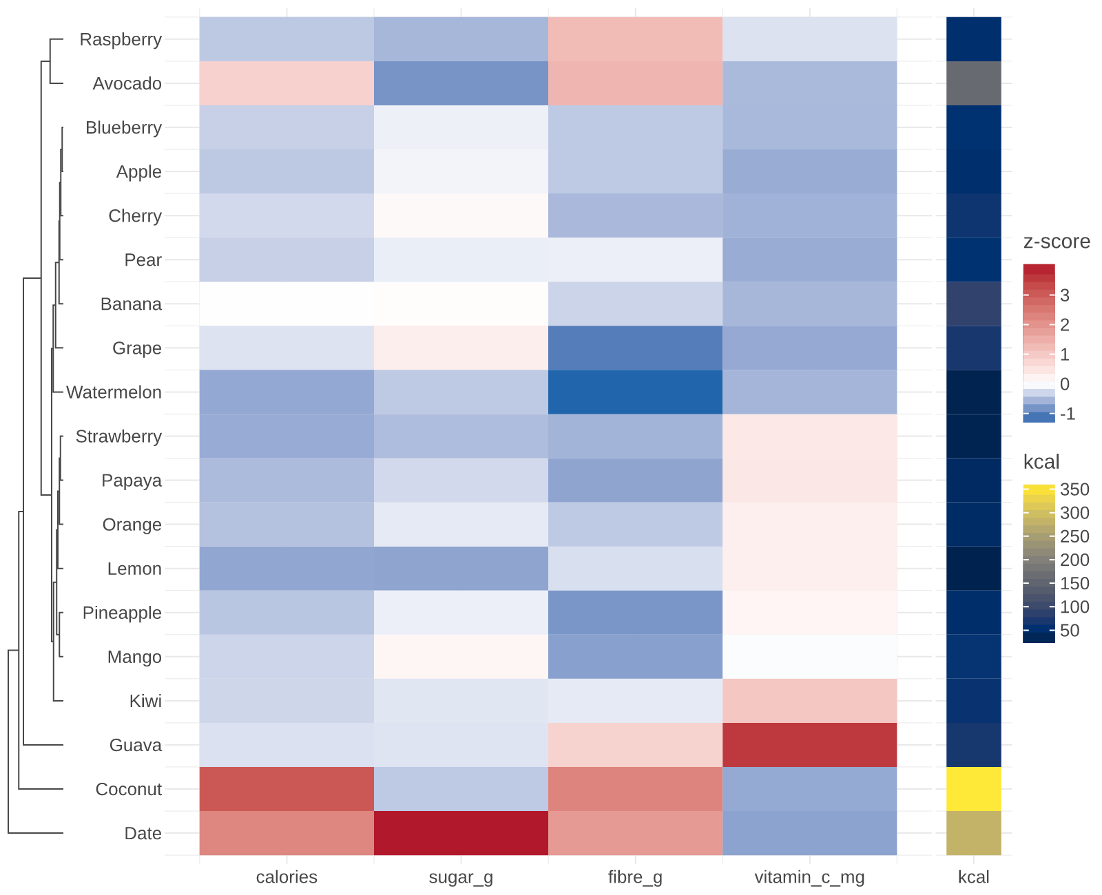
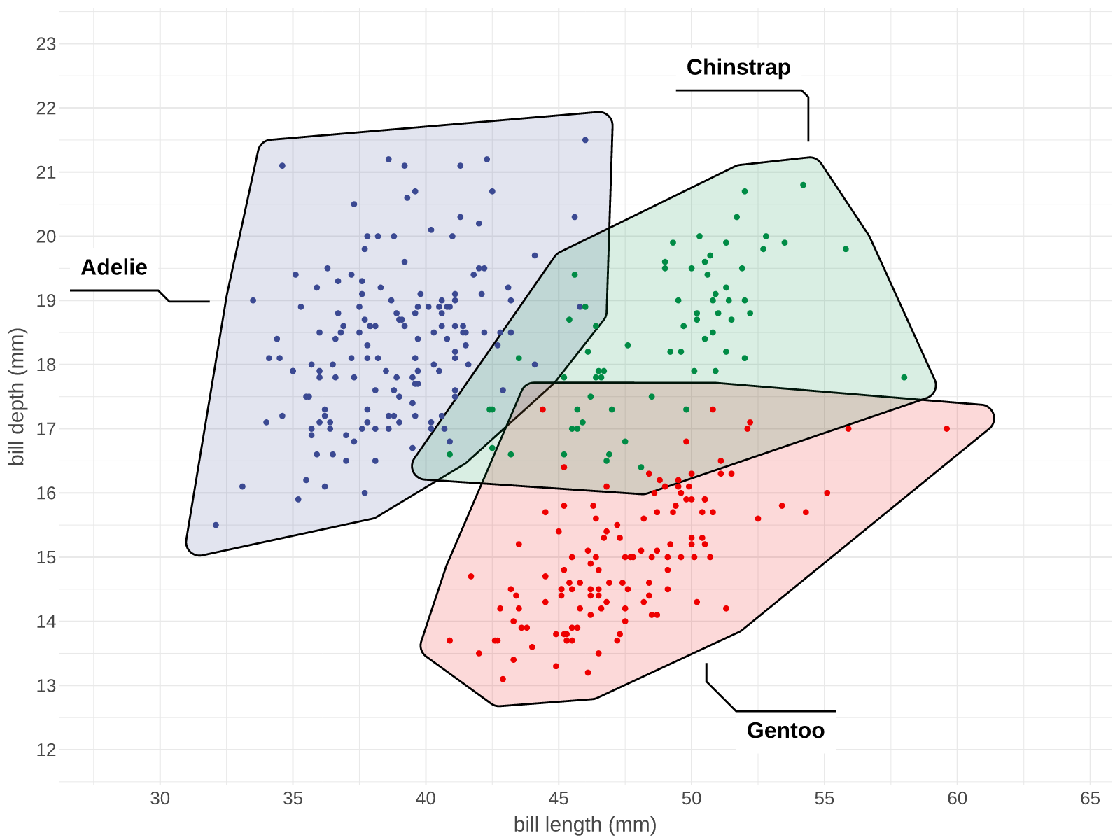
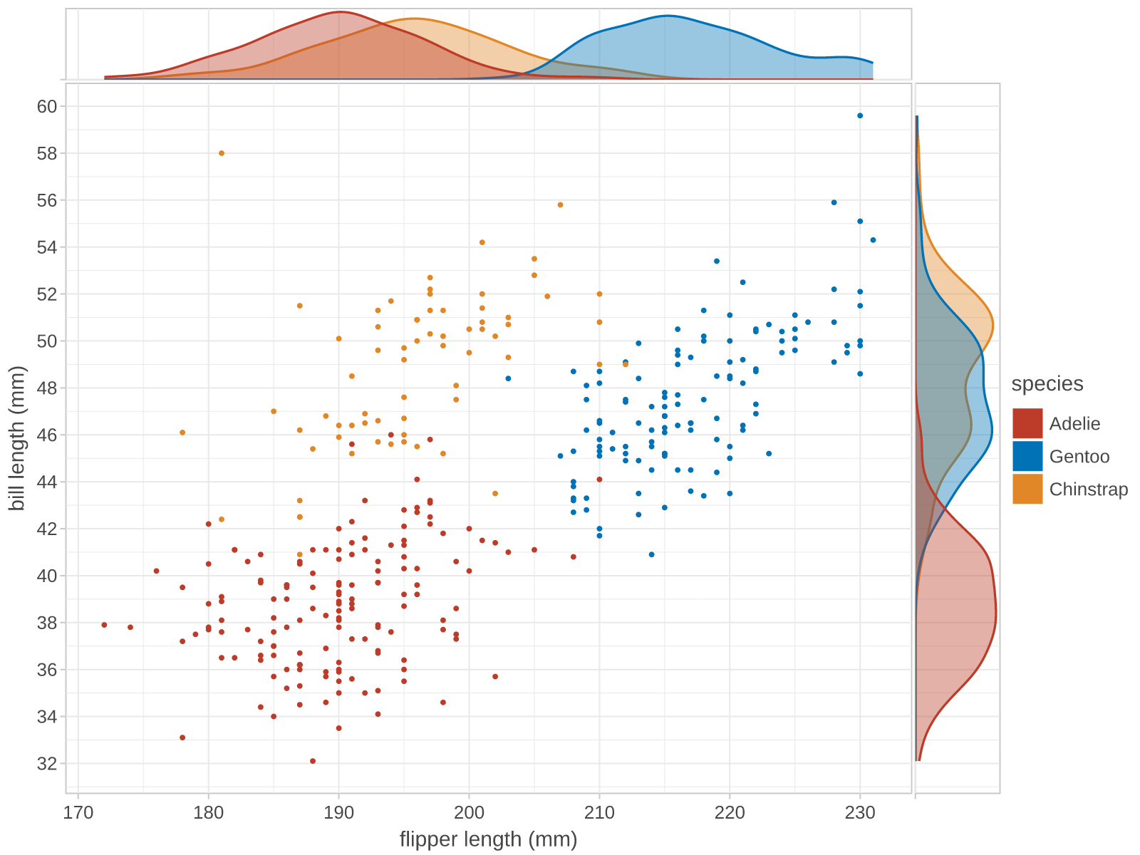
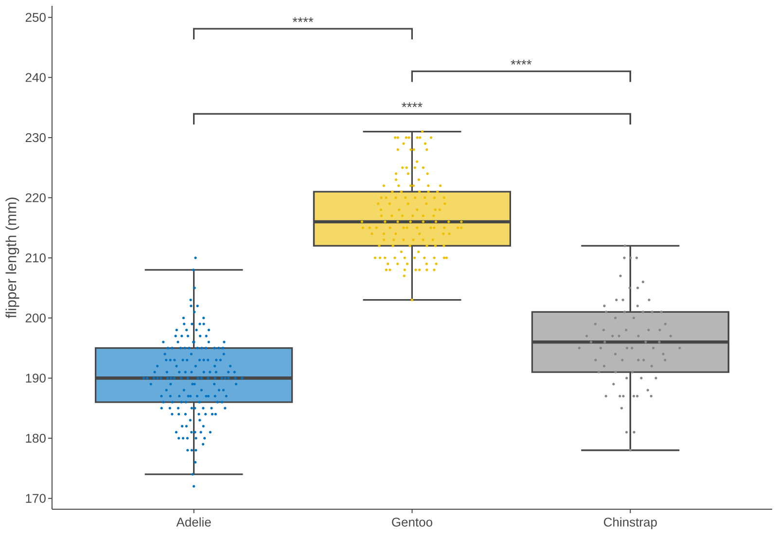
Every plot above is ggrust. More in the gallery.
- Fast and lean: at 1M rows a typical plot renders 5x faster than ggplot2 and 90x faster than Lets-Plot, with 4x and 7.5x less memory (benchmarks).
- ggplot2 extensions, built in: beeswarms, significance brackets, cluster marks, side panels, dendrograms, raincloud plots, patchwork layouts and more, under their R names (list).
- The Lets-Plot API: most code ports with an import swap,
lets_plot->ggrust. - Interactive: notebook and HTML output with tooltips, zoom and pan; dense point layers drawn on a canvas.
- Publication output: SVG, PNG, vector PDF and HTML, with your own fonts. Data crosses into Rust once, as Arrow, so Polars and pandas frames work directly.
pip install ggrustuv add ggrustimport polars as pl
from ggrust import *
frame = pl.DataFrame(
{
"height": [150, 162, 171, 180, 168, 175],
"weight": [52, 60, 68, 82, 65, 74],
"group": ["a", "a", "b", "b", "c", "c"],
}
)
plot = (
ggplot(frame, aes(x="height", y="weight", color="group"))
+ geom_point(size=4)
+ labs(title="Height vs weight")
+ ggsize(600, 400)
)
plot.to_png("plot.png")
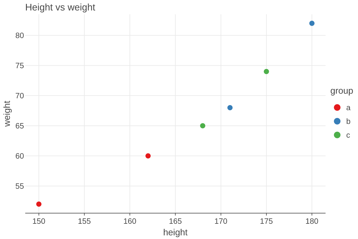
In a notebook the plot shows as interactive HTML (tooltips, zoom and pan with ggtb()).
Many popular ggplot2 extension packages from R are built into ggrust, under their R function names. Nothing extra to install; Lets-Plot has none of them.
| Feature | ggrust | From the R package |
|---|---|---|
| Beeswarm and quasirandom points | geom_beeswarm, geom_quasirandom |
ggbeeswarm |
| Journal color palettes | scale_color_npg, _aaas, _nejm, _lancet, _jama, _jco, _d3, _igv |
ggsci |
| Significance tests and labels | stat_compare_means, stat_cor, stat_poly_eq |
ggpubr, ggpmisc |
| Cluster marks | geom_mark_hull, geom_mark_ellipse, geom_mark_rect |
ggforce |
| Highlighting | gghighlight |
gghighlight |
| Point density | geom_pointdensity |
ggpointdensity |
| Side panels | geom_xside*, geom_yside*, ggmarginal |
ggside |
| Several color scales in one plot | new_scale_fill, new_scale_color, new_scale |
ggnewscale |
| Dendrograms | hclust, scale_x_dendro, scale_y_dendro, geom_dendrogram |
legendry, ggh4x, ggdendro |
| Raincloud plots | stat_halfeye, stat_interval, geom_half_violin, geom_half_boxplot, geom_half_point |
ggdist, gghalves |
| Figure layouts and panel tags | gggrid(design=, tag_levels=), inset_element |
patchwork |
| Rasterized layers in vector output | rasterize |
ggrastr, scattermore |
ggrust reimplements their behavior in Rust; the R packages and their authors designed it. Examples and credits are in the extensions guide.
11 everyday plots (scatter, histogram, boxplot, violin, density, lm smooth, line, 2D bins, facets and more) at 10k, 100k and 1M rows, each saved as SVG and PNG. Same data, every row drawn (Lets-Plot's sampling turned off), same output size, each run in a fresh process. Apple M4 Pro; ggrust main (0.8.0 plus a line-drawing fix), R ggplot2 4.0.1 (svglite, ragg), lets-plot 4.11.0.
| 1M rows | SVG, all 11 plots | PNG, all 11 plots | peak memory per plot |
|---|---|---|---|
| ggrust | 0.91 s | 2.85 s | 138 MB |
| ggplot2 | 9.67 s (10.6x) | 25.0 s (8.8x) | 560 MB |
| Lets-Plot | 71.6 s (78.9x) | > 495 s (> 174x) | 1.0 GB |
- ggrust is faster than both in all 66 cases (11 plots x 3 sizes x 2 formats).
- Lets-Plot did not finish the 1M-row line PNG within 300 s; it counts as 300 s in its total.
Charts, rules and how to reproduce: the benchmarks page. Raw numbers: benchmarks/REPORT-three-way.md.
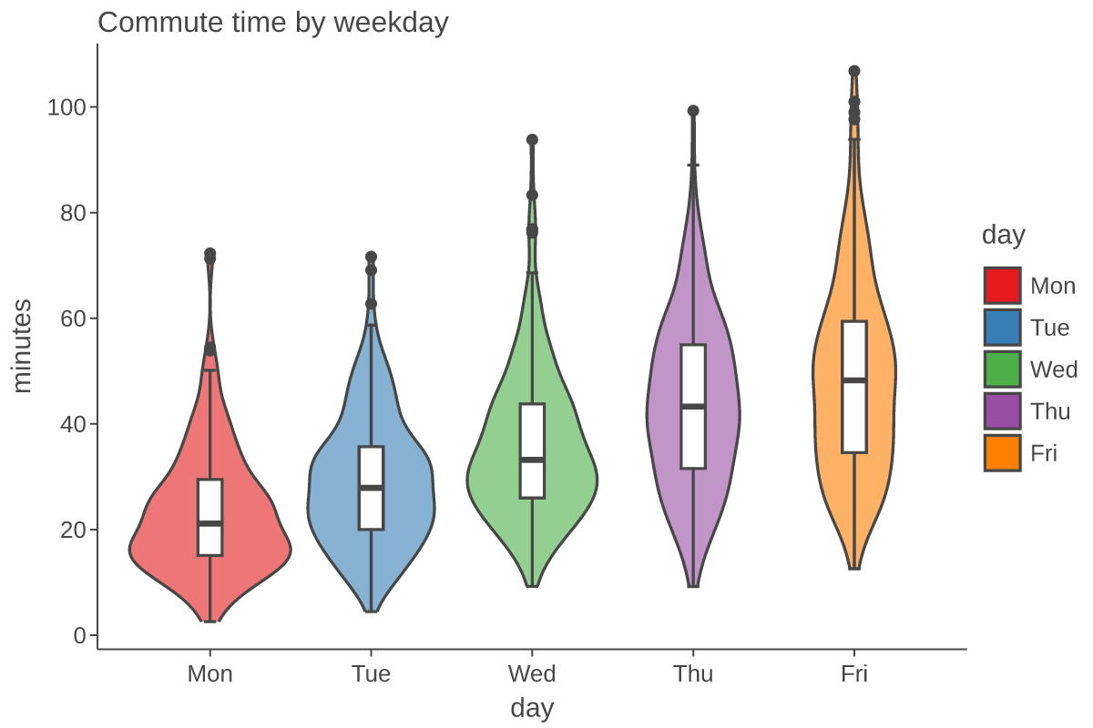
Violins with boxplots on top, using the same layering as ggplot.
Show code
import numpy as np

rng = np.random.default_rng(0)
days = ["Mon", "Tue", "Wed", "Thu", "Fri"]
commute = pl.DataFrame(
    {
        "day": np.repeat(days, 200),
        "minutes": np.concatenate([rng.gamma(4 + i, 6, 200) for i in range(5)]),
    }
)

(
    ggplot(commute, aes(x="day", y="minutes", fill="day"))
    + geom_violin(alpha=0.6)
    + geom_boxplot(width=0.15, fill="white")
    + labs(title="Commute time by weekday")
    + theme_classic()
    + ggsize(600, 400)
)
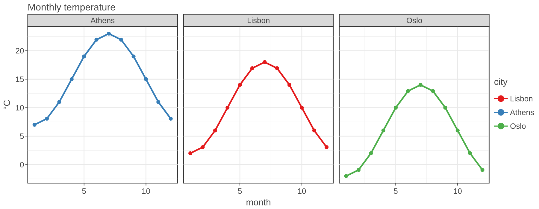
Split a plot into panels by a column.
Show code
months = np.arange(1, 13)
temperature = pl.DataFrame(
    {
        "month": np.tile(months, 3),
        "temp": np.concatenate(
            [10 + 8 * np.sin((months - 3) / 12 * 2 * np.pi) + offset for offset in (0, 5, -4)]
        ),
        "city": np.repeat(["Lisbon", "Athens", "Oslo"], 12),
    }
)

(
    ggplot(temperature, aes(x="month", y="temp", color="city"))
    + geom_line(size=1.2)
    + geom_point()
    + facet_wrap("city", ncol=3)
    + labs(title="Monthly temperature", y="°C")
    + theme_bw()
    + ggsize(900, 350)
)
- Geoms: point, line, path, bar, col, histogram, boxplot, violin, area ridges, tile, raster, rect, text, label, text/label repel, segment, curve, polygon, rug, imshow, brackets and more.
- Stats: count, bin, density, smooth, summary, ecdf, contours, 2D bins, ellipses.
- Scales: continuous, discrete, log, reversed, datetime, hue, manual, gradients, viridis, brewer, secondary axes, axes on any side.
- Layout:
facet_wrap,facet_grid,gggridwith collected legends,coord_fixed,coord_flip, themes (theme_classic,theme_bw,theme_minimal,theme_void, ...). - Outputs: SVG, PNG, vector PDF, and interactive HTML through
ggsave, with your own fonts (register_font). Dense scatter layers are drawn on a canvas in HTML.
ggrust is a subset of Lets-Plot, not all of it. Features follow what Cellestial and everyday plotting need. See the migration note for the differences.
Early, but usable: the full Cellestial test suite passes on ggrust. Expect rough edges and API gaps; issues are welcome.
uv sync          # create the dev environment
make develop     # build the Rust extension into .venv
make check       # fmt, clippy, ruff, cargo test, pytest