Waveguide

Calculate the various properties of rectangular waveguides

For example:

• Cutoff frequency of various modes
• Attenuation due to conductor and/or dielectric loss
• Surface resistance and skin depth
• Effective conductivity at cryogenic temperatures (anomalous skin effect)
• Properties of waveguide cavities: resonant frequency, Q-factor

Example 1: Properties of a WR-90 Waveguide

WR-90 waveguide:

import numpy as np 
import scipy.constants as sc
import matplotlib.pyplot as plt
from waveguide import phase_constant, attenuation_constant

# WR-90 waveguide dimensions
a, b = 0.9 * sc.inch, 0.45 * sc.inch

# Conductivity of waveguide walls, S/m
cond = 2e7

# Frequency sweep
freq = np.linspace(7, 13, 100) * sc.giga

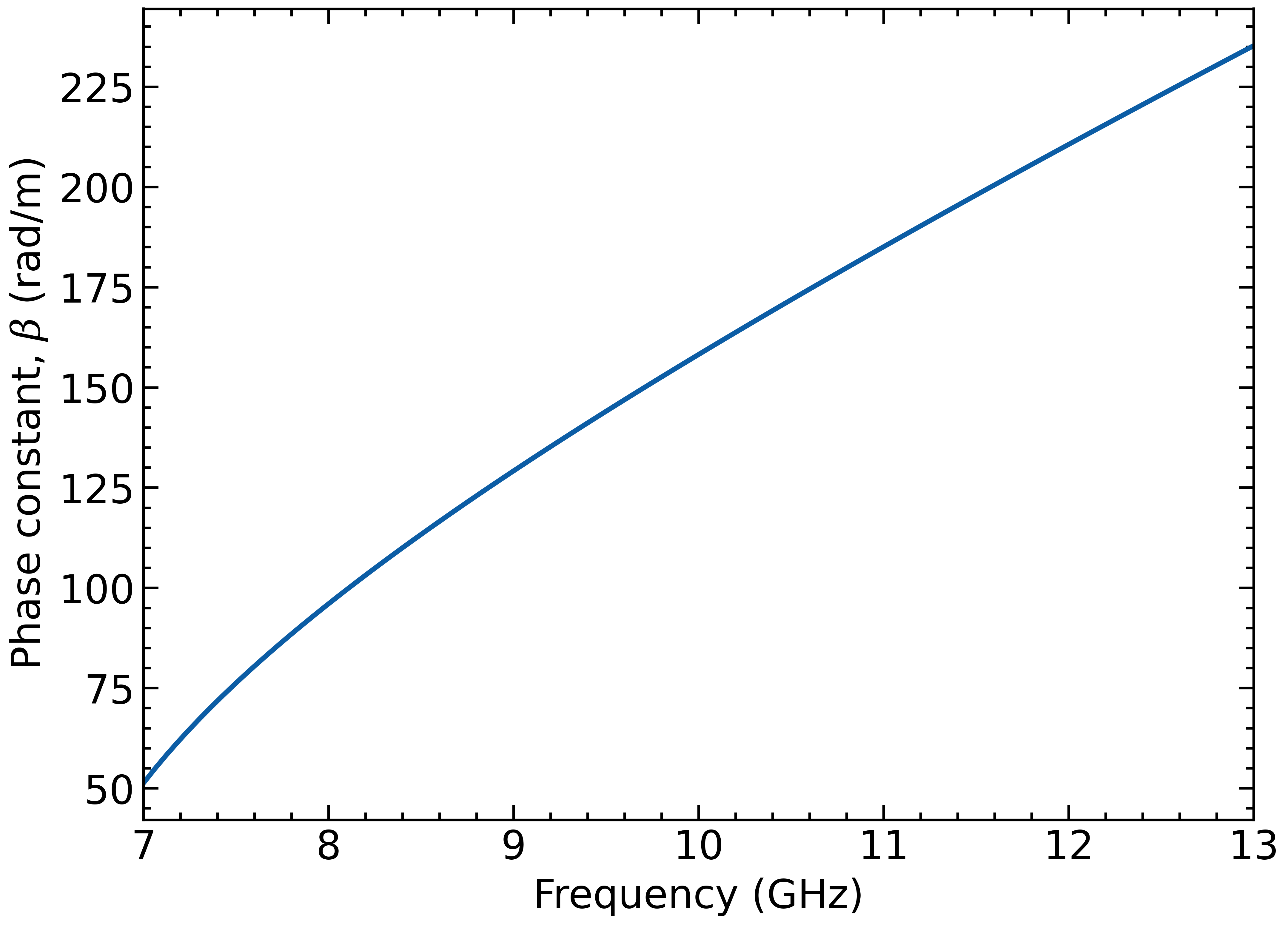
Phase constant:

beta = phase_constant(freq, a, b, cond=cond)

plt.figure()
plt.plot(freq/1e9, beta)
plt.ylabel(r"Phase constant, $\beta$ (rad/m)")
plt.xlabel("Frequency (GHz)")
plt.xlim([7, 13])

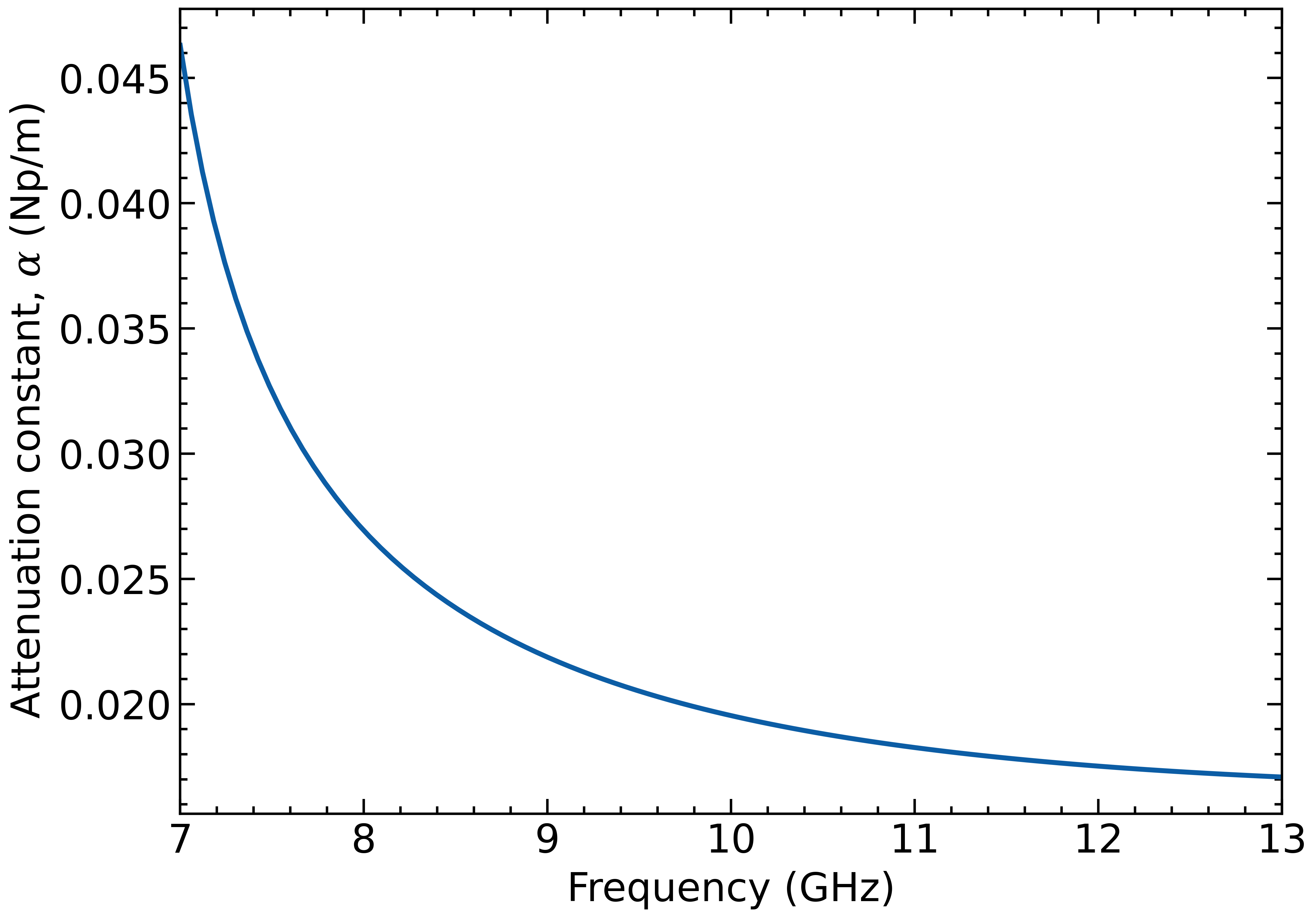
Attenuation constant:

alpha = attenuation_constant(freq, a, b, cond=cond)

plt.figure()
plt.plot(freq/1e9, alpha)
plt.ylabel(r"Attenuation constant, $\alpha$ (Np/m)")
plt.xlabel("Frequency (GHz)")
plt.xlim([7, 13])

Example 2: Cutoff Frequencies

import numpy as np
import scipy.constants as sc
from waveguide import cutoff_frequency

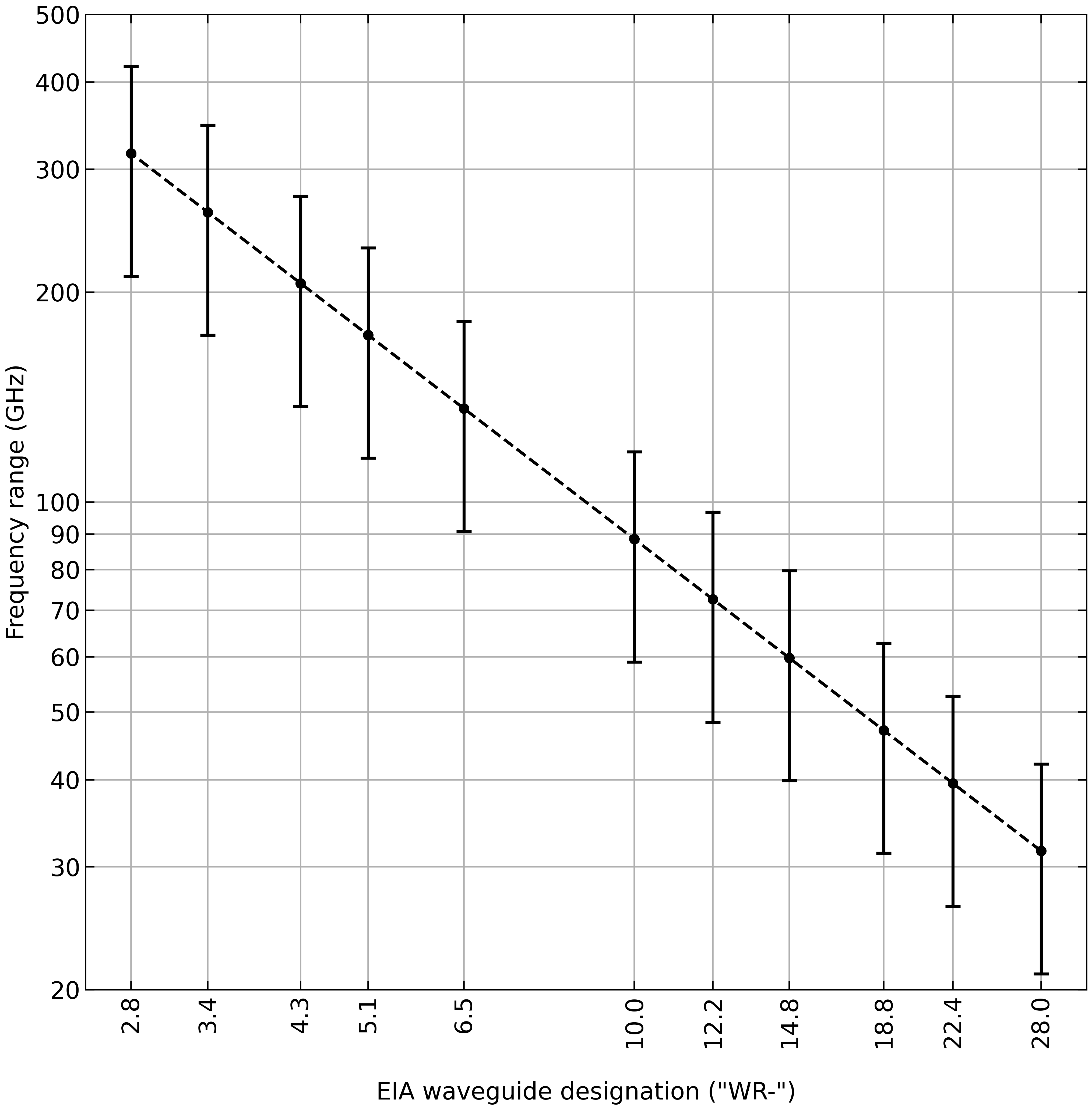
# Waveguide sizes to analyze (EIA designations)
wr_sizes = np.array([28, 22.4, 18.8, 14.8, 12.2, 10, 6.5, 5.1, 4.3, 3.4, 2.8])

# Calculate cutoff frequencies
f_center = np.empty_like(wr_sizes)
f1 = np.empty_like(wr_sizes)
f2 = np.empty_like(wr_sizes)
for i, _wr in np.ndenumerate(wr_sizes):
    a = _wr * 10 * sc.mil  # waveguide width
    f1[i] = cutoff_frequency(a, a/2, m=1, n=0) * 1.25  # TE10
    f2[i] = cutoff_frequency(a, a/2, m=2, n=0) * 0.95  # TE20
    f_center[i] = (f1[i] + f2[i]) / 2

# Plot    
fig, ax = plt.subplots(figsize=(12,12))
ax.loglog(wr_sizes, f_center/1e9, 'ko')
ax.errorbar(wr_sizes, f_center/1e9, yerr=[(f_center-f1)/1e9, -(f_center-f2)/1e9], c='k', fmt='o', ls='--', capsize=5, capthick=2)
ax.set_xlabel("\nEIA waveguide designation (\"WR-\")")
ax.set_ylabel("Frequency range (GHz)")
ax.set_ylim([20, 500])
ax.grid(which='both')
plt.yticks(ticks=[20, 30, 40, 50, 60, 70, 80, 90, 100, 200, 300, 400, 500], 
           labels=[20, 30, 40, 50, 60, 70, 80, 90, 100, 200, 300, 400, 500])
ax.set_xticks(ticks=wr_sizes, minor=False)
ax.set_xticks(ticks=[], minor=True)
plt.xticks(ticks=wr_sizes, labels=wr_sizes, rotation=90)

Example 3: Alumina-Filled WR-28 Waveguide

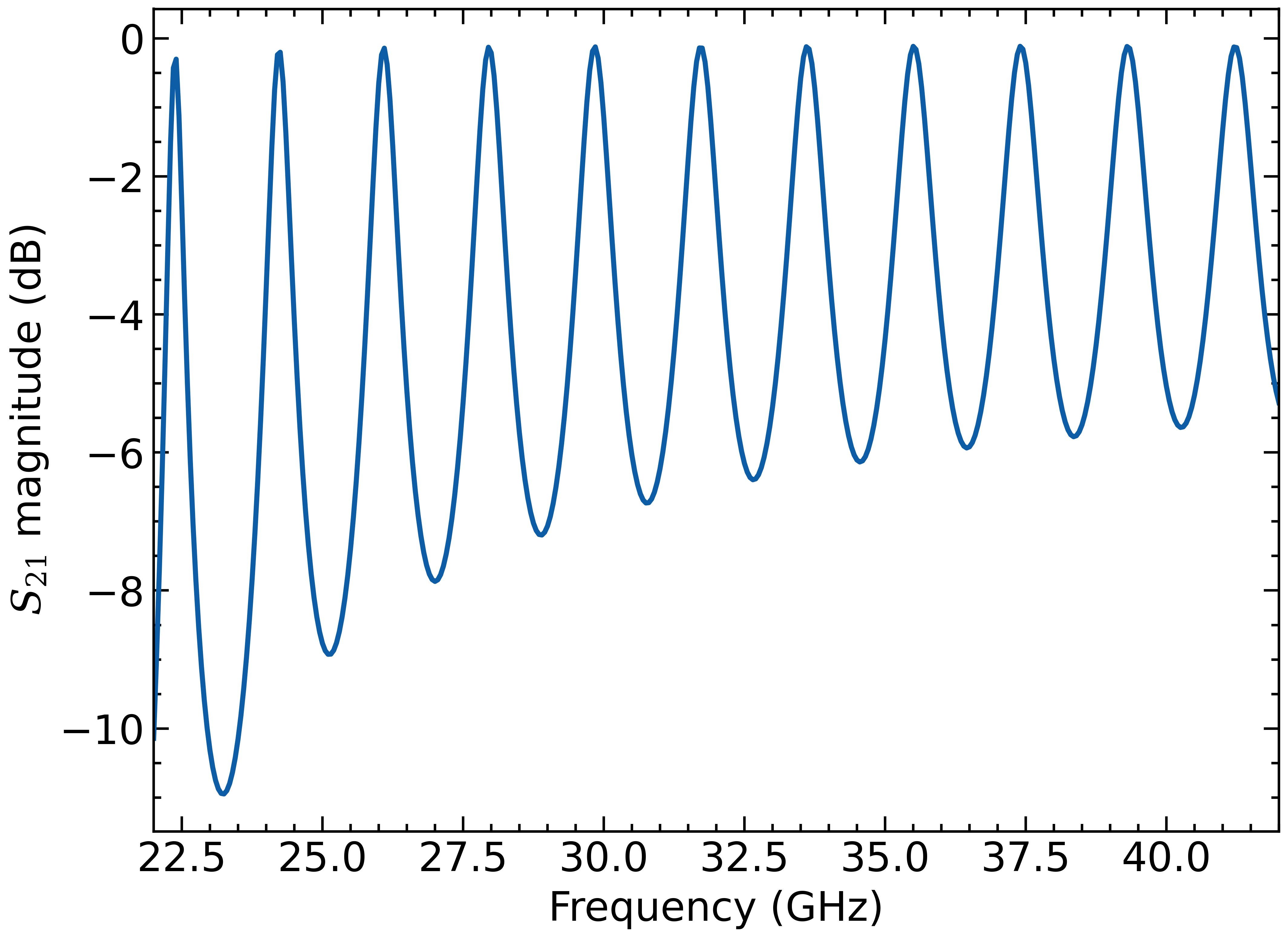
WR-28 waveguide filled with 1 inch long alumina slug:

import numpy as np 
import scipy.constants as sc
import matplotlib.pyplot as plt 

import waveguide as wg

# WR-28 waveguide dimensions
a, b = 0.28 * sc.inch, 0.14 * sc.inch

# Conductivity of waveguide walls, S/m
cond = 1.8e7

# Frequency sweep
freq = np.linspace(22, 42, 401) * sc.giga

# Relativity permittivity
er = 9.3

# Alumina length, m
length = 1 * sc.inch

# Section lengths
total_length = 1.7 * sc.inch
length1 = (total_length - length) / 2
length2 = length
length3 = length1

# S-parameters
_, _, s21, _ = wg.dielectric_sparam(freq, a, b, er, 0, cond, length1, length2, length3)

fig, ax = plt.subplots()
ax.plot(freq/1e9, 20*np.log10(np.abs(s21)))
plt.ylabel(r"$S_{21}$ magnitude (dB)")
plt.xlabel("Frequency (GHz)")
plt.xlim([22, 42])

References

The equations in this package are taken from:

• D. M. Pozar, Microwave Engineering, 4th ed. John Wiley & Sons, Inc., 2011.

• N. Marcuvitz, Waveguide Handbook. McGraw-Hill Book Company, Inc., 1951.